Fluorescence In Situ Sequencing (FISSEQ)
26th of October - Evan Daugharthy (Harvard) + George Church (Harvard)
Slides Recordings Note: Please do not distribute the slides outside of class, thanks!!
Introduction
Why do we need analytic tools for synthetic projects? The tools for synthetic biology have grown incredibly powerful: DNA synthesis, genome engineering, synthetic cells, directed evolution, cell-free systems, metabolic engineering, and nanomaterial science. However, these tools only cover the second half of the “read/write” cycle. In this class, we will discuss the rationale for developing measurement technologies (“read”) to complement these engineering tools (“write”), so that we can understand the effects of our bioengineering efforts and make new products that resemble real biological systems.
We will review various approaches to molecular measurements, including DNA and RNA sequencing, proteomics, and 3D structural morphometry. We will focus predominantly on in situ detection of single molecules (in situ is latin for “in place,” referring to detection of molecules inside cells). Finally, we will discuss applications of these technologies to fibroblast wound healing, understanding how the brain works, and to developing new organoids to further our understanding of biological development and create new biomedical interventions to advance human health.
Readings
Background Reading:
The FISSEQ Method: Lee J, Daugharthy E, Scheiman J, Kalhor R, Yang JL, Ferrente TC, Terry R, Jeanty SSF, Li C,Amamoto R, Peters DT, Turczyk BM, Marblestone A, Inverso S, Bernard A, Mali P, Rios X, Aach J, Church GM (2014) Highly multiplexed three-dimensional subcellular transcriptome sequencing in situ. Science 343(6177):1360-3.
Theory of RNA and Cellular Molecular State: Kim, Junhyong, and James Eberwine (2010) RNA: state memory and mediator of cellular phenotype. Trends in cell biology 20.6:311-318.
Additional Reviews of FISSEQ and Single-Cell Sequencing
Ginart, Paul, and Arjun Raj (2014) RNA sequencing in situ. Nature biotechnology 32.6:543-544.
Mignardi, Marco, and Mats Nilsson (2014) Fourth-generation sequencing in the cell and the clinic. Genome medicine 6.4:31.
Avital, Gal, Tamar Hashimshony, and Itai Yanai (2014) Seeing is believing: new methods for in situ single-cell transcriptomics. Genome biology 15.3:110.
Additional Theory
Eberwine, James, and Junhyong Kim (2015) Cellular Deconstruction: Finding Meaning in Individual Cell Variation. Trends in cell biology 25.10:569-578.
Trapnell, Cole (2015) Defining cell types and states with single-cell genomics. Genome research 25.10:1491-1498.
Additional Historical Context of DNA Sequencing
Hutchison, Clyde A. (2007) DNA sequencing: bench to bedside and beyond. Nucleic acids research 35.18: 6227-6237.
Goodwin, Sara, John D. McPherson, and W. Richard McCombie. (2016) Coming of age: ten years of next-generation sequencing technologies. Nature Reviews Genetics 17.6: 333-351.
Homework
Although the complexity and expense of biological measurement technologies continues to fall, this homework may still be quite challenging. The assignment is comprised of several aspects:
- Experimental design
- Computational analysis
- Bench “wet” work
Please attempt to complete all three aspects!
For the bench work, I appreciate that this may be very challenging in a DIY space, so the bench work contains several versions of the homework that vary in difficulty. Please work towards the increasingly challenging homework until you reach the limits of your facility.
If challenges may arise the computational aspects, such as poor documentation, bugs, version incompatibilities, and hardware limitations, please use the resources available on the Internet to help you. Stack Overflow is a great resource for advice on programming, and a quick Google search is always a good first line of inquiry.
As the price of DNA sequencing continues to fall and the Bio Academy continues to grow, we anticipate that HTGAA participants will be able to conduct simple genome sequencing experiments within a few years! Your effort and feedback with this project are crucial to help us understand what is feasible in a DIY Bio space!
Grading
To be considered “passing” this assignment, please complete the following tasks:
- Group discussion about the Experimental Design questions.
- Individual or group written answers to all four Experimental Design questions (note which people contributed to each submission). See guidelines for answering in that section.
- Go through the entire Introduction to Image Processing Assignment tutorial.
- Identify the nuclei of this FISSEQ image using the tools from the tutorial.
- Go through the entire Introduction to Bioinformatics tutorial (show the phylogenetic tree output from the final step).
- Use Biopython to convert a DNA sequencing into the corresponding RNA and protein sequence (for help see the Bio.Seq module).
- Read the Experimental Assignments section.
Experimental Design Assignment
Feel free to pull answers from the slide deck, but also use Google, Wikipedia, or online scientific publications to gather other perspectives. Think back to your experience so far with HTGAA to think of experiments where in situ data of RNA, DNA, protein, or other cellular features would be helpful in understanding the engineering process. If it is helpful, use a specific application or synthetic biology goal to inspire your answers.
Answer the following questions:
- What are some reasons in situ data could be better than bulk data for this experiment? Try to think of cases where a bulk measurement would cause you to miss some insight.
- What kinds of molecules would you like to detect? E.g. what species of RNA? How could you build a list of molecules that would be relevant? How would you go about targeting those molecules?
- What limits your ability to detect the things you are interested in?
- What limits are imposed by physics on the resolution of light/fluorescence microscopy? What is one strategy to overcome this?
- Try to think of another limit imposed by the laws of physics, and describe how it limits measurement.
- We only want to measure properties of biological systems that exhibit meaningful variation. For example, if you go all the way down to sub-atomic particles, biological systems probably look pretty similar. Make an argument for a “specification” of an ideal measurement—e.g. that no one would want to acquire the measurement more precisely. Consider space, time, or physical composition.
Try to be as detailed as possible and think creatively! You should be able to write a couple sentences about each answer. These are the kinds of questions we ask every day and that come up as we talk to other scientists who want to use FISSEQ. These questions drive our technology development process!
Computational Assignments
Everyone should be able to complete the two introductory assignments. If you have a powerful computer and have access to MATLAB software, you might also try the final advanced assignment.
Required Assignment: Introduction to Image Processing
(Adapted from Python Image Tutorial)
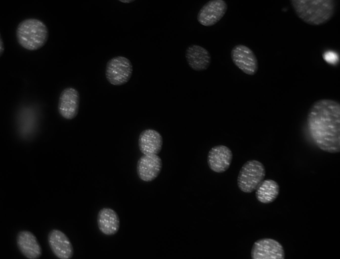
As you have seen, the FISSEQ method generates image data, which must be analyzed. One image analysis task we performed in the original paper was to identify the nuclei so that we could determine whether each RNA molecule was localized to the nucleus or cytoplasm. In this homework, you will segment an image of a nuclear stain.
Install the following software:
- Python 2.5, 2.6, or 2.7
- numpy
- matplotlib
- mahotas
- ipython
Under Linux, you can just install your distribution’s packages (install at least python-numpy, python-numpy-dev, python-matplotlib, ipython). Under Windows or Mac OS, you can use the Anaconda Distribution (use Python 2.7) (actually this works on Linux too, if you prefer this method).
First Task: Counting Nuclei
Download the image. Before we start, let us import the needed files. For all code examples in this tutorial, I am going to assume that you typed the following before coming to the example:
import numpy as np
import pylab
import mahotas as mh
These are the packages listed above (except pylab, which is a part of matplotlib).
In Python, there is image processing tools spread across many packages instead of a single package. Fortunately, they all work on the same data representation, the numpy array 1). A numpy array is, in our case, either a two dimensional array of integers (height x width) or, for colour images, a three dimensional array (height x width x 3 or height x width x 4, with the last dimension storing (red,green,blue) triplets or (red,green,blue,alpha) if you are considering transparency).
The first step is to get the image from disk into a memory array:
dna = mh.imread('dna.jpeg')
In interactive mode (i.e., if you are running this inside ipython), you can see the image:
pylab.imshow(dna)
pylab.show()
If you set up things in a certain way, you might not need the pylab.show() line. For most installations, you can get this by running ipython -pylab on the command line 2).
You might be surprised that the image does not look at all like the one above.
This is because, by default, pylab shows images as a heatmap. You can see the more traditional grey-scale image by switching the colormap used. Instead of the default jet colourmap, we can set it to the gray one, which is the traditional greyscale representation:
pylab.imshow(dna)
pylab.gray()
pylab.show()
We can explore our array a bit more:
print dna.shape
print dna.dtype
print dna.max()
print dna.min()
Since dna is just a numpy array, we have access to all its attributes and methods (see the numpy documentation for complete information).
The above code prints out:
(1024, 1344)
uint8
252
0
The shape is 1024 pixels high and 1344 pixels across (recall that the convention is the matrix convention: height x width). The type is uint8, i.e., unsigned 8-bit integer. The maximum value is 252 and the minimum value is 0 3).
pylab.imshow(dna // 2)
pylab.show()
Here, we are displaying an image where all the values have been divided by 2 4). And the displayed image is still the same! In fact, pylab contrast-stretches our images before displaying them.
Here’s the first idea for counting the nuclei. We are going to threshold the image and count the number of objects.
T = mh.thresholding.otsu(dna)
pylab.imshow(dna > T)
pylab.show()
Here, again, we are taking advantage of the fact that dna is a numpy array and using it in logical operations (dna > T). The result is a numpy array of booleans, which pylab shows as a black and white image (or red and blue if you have not previously called pylab.gray()).
This isn’t too good. The image contains many small objects. There are a couple of ways to solve this. A simple one is to smooth the image a bit using a Gaussian filter.
dnaf = mh.gaussian_filter(dna, 8)
T = mh.thresholding.otsu(dnaf)
pylab.imshow(dnaf > T)
pylab.show()
The function mh.gaussian_filter takes an image and the standard deviation of the filter (in pixel units) and returns the filtered image. We are jumping from one package to the next, calling mahotas to filter the image and to compute the threshold, using numpy operations to create a thresholded images, and pylab to display it, but everyone works with numpy arrays. The result is much better.
We now have some merged nuclei (those that are touching), but overall the result looks much better. The final count is only one extra function call away:
labeled,nr_objects = mh.label(dnaf > T)
print nr_objects
pylab.imshow(labeled)
pylab.jet()
pylab.show()
We now have the number of objects in the image (18), and we also displayed the labeled image. The call to pylab.jet() just resets the colourmap to jet if you still had the greyscale map active.
We can explore the labeled object. It is an integer array of exactly the same size as the image that was given to mh.label(). It’s value is the label of the object at that position, so that values range from 0 (the background) to nr_objects.
Second Task: Segmenting the Image
The previous result was acceptable for a first pass, but there were still nuclei glued together. Let’s try to do better.
Here is a simple, traditional, idea:
- smooth the image
- find regional maxima
- use the regional maxima as seeds for watershed
1. Finding the seeds
Here’s our first try:
dnaf = mh.gaussian_filter(dna, 8)
rmax = mh.regmax(dnaf)
pylab.imshow(mh.overlay(dna, rmax))
pylab.show()
The mh.overlay() returns a colour image with the grey level component being given by its first argument while overlaying its second argument as a red channel. The result doesn’t look so good. If we look at the filtered image, we can see the multiple maxima. After a little fiddling around, we decide to try the same idea with a bigger sigma value:
dnaf = mh.gaussian_filter(dna, 16)
rmax = mh.regmax(dnaf)
pylab.imshow(mh.overlay(dna, rmax))
Now things look much better.
We can easily count the number of nuclei now:
seeds,nr_nuclei = mh.label(rmax)
print nr_nuclei
Which now prints 22.
2. Watershed
We are going to apply watershed to the distance transform of the thresholded image:
T = mh.thresholding.otsu(dnaf)
dist = mh.distance(dnaf > T)
dist = dist.max() - dist
dist -= dist.min()
dist = dist/float(dist.ptp()) * 255
dist = dist.astype(np.uint8)
pylab.imshow(dist)
pylab.show()
After we contrast stretched the dist image, we can call mh.cwatershed to get the final result [^5] (the colours in the image come from it being displayed using the jet colourmap):
nuclei = mh.cwatershed(dist, seeds)
pylab.imshow(nuclei)
pylab.show()
It’s easy to extend this segmentation to the whole plane by using generalised Voronoi (i.e., each pixel gets assigned to its nearest nucleus):
whole = mh.segmentation.gvoronoi(nuclei)
pylab.imshow(whole)
pylab.show()
Often, we want to provide a little quality control and remove those cells whose nucleus touches the border. So, let’s do that:
borders = np.zeros(nuclei.shape, np.bool)
borders[ 0,:] = 1
borders[-1,:] = 1
borders[:, 0] = 1
borders[:,-1] = 1
at_border = np.unique(nuclei[borders])
for obj in at_border:
    whole[whole == obj] = 0
pylab.imshow(whole)
pylab.show()
This is a bit more advanced, so let’s go line by line:
borders = np.zeros(nuclei.shape, np.bool)
This builds an array of zeros, with the same shape as nuclei and of type np.bool.
borders[ 0,:] = 1
borders[-1,:] = 1
borders[:, 0] = 1
borders[:,-1] = 1
This sets the borders of that array to True (1 is often synonymous with True).
at_border = np.unique(nuclei[borders])
nuclei[borders] gets the values that the nuclei array has where borders is True (i.e., the value at the borders), then np.unique returns only the unique values (in our case, it returns array([ 0, 1, 2, 3, 4, 6, 8, 13, 20, 21, 22])).
for obj in at_border:
    whole[whole == obj] = 0
Now we iterate over the border objects and everywhere that whole takes that value, we set it to zero 5). We now get our final result.
Learn More
You can explore the documentation for numpy at docs.numpy.org. You will find documentation for scipy at the same location. For mahotas, you can look at its online documentation.
However, Python has a really good online documentation system. You can invoke it with help(name) or, if you are using ipython just by typing a question mark after the name of the function you are interested in, e.g.,
In [2]: mh.regmax?
Required Assignment: Introduction to Bioinformatics
(Adapted from BioPython Basics and Guide to Bioinformatics with BioPython)
Scientists use computational tools to store, manipulate, model, and compute on biological data. From the biopython website their goal is to “make it as easy as possible to use Python for bioinformatics by creating high-quality, reusable modules and scripts.” These modules use the biopython tutorial as a template for what you will learn here. Here is a list of some of the most common data formats in computational biology that are supported by biopython.
| Uses | Note |
|---|---|
| Blast | finds regions of local similarity between sequences |
| ClustalW | multiple sequence alignment program |
| GenBank | NCBI sequence database |
| PubMed and Medline | Document database |
| ExPASy | SIB resource portal (Enzyme and Prosite) |
| SCOP | Structural Classification of Proteins (e.g. ‘dom’,’lin’) |
| UniGene | computationally identifies transcripts from the same locus |
| SwissProt | annotated and non-redundant protein sequence database |
Some of the other principal functions of biopython.
- A standard sequence class that deals with sequences, ids on sequences, and sequence features.
- Tools for performing common operations on sequences, such as translation, transcription and weight calculations.
- Code to perform classification of data using k Nearest Neighbors, Naive Bayes or Support Vector Machines.
- Code for dealing with alignments, including a standard way to create and deal with substitution matrices.
- Code making it easy to split up parallelizable tasks into separate processes.
- GUI-based programs to do basic sequence manipulations, translations, BLASTing, etc.
Getting Started
Download and install Biopython. In python, import the Biopython module.
>>> import Bio
>>> Bio.__version__
'1.58'
Some examples will also require a working internet connection in order to run.
>>> from Bio.Seq import Seq
>>> my_seq = Seq("AGTACACTGGT")
>>> my_seq
Seq('AGTACACTGGT', Alphabet())
>>> aStringSeq = str(my_seq)
>>> aStringSeq
'AGTACACTGGT'
>>> my_seq_complement = my_seq.complement()
>>> my_seq_complement
Seq('TCATGTGACCA', Alphabet())
>>> my_seq_reverse = my_seq.reverse()
>>> my_seq_rc = my_seq.reverse_complement()
>>> my_seq_rc
Seq('ACCAGTGTACT', Alphabet())
There is so much more, but first before we get into it we should figure out how to get sequences in and out of python. Download this FASTA file.
FASTA formats are the standard format for storing sequence data. Here is a little reminder about sequences.
| Nucleic acid code | Note | Nucleic acid code | Note |
|---|---|---|---|
| A | adenosine | K | G/T (keto) |
| T | thymidine | M | A/C (amino) |
| C | cytidine | R | G/A (purine) |
| G | guanine | S | G/C (strong) |
| N | A/G/C/T (any) | W | A/T (weak) |
| U | uridine | B | G/T/C |
| D | G/A/T | Y | T/C (pyrimidine) |
| H | A/C/T | V | G/C/A |
Here is quickly a bit about how biopython works with sequences:
>>> for seq_record in SeqIO.parse(os.path.join("data","ls_orchid.fasta"), "fasta"):
...     print seq_record.id
...     print repr(seq_record.seq)
...     print len(seq_record)
...
gi|2765658|emb|Z78533.1|CIZ78533
Seq('CGTAACAAGGTTTCCGTAGGTGAACCTGCGGAAGGATCATTGATGAGACCGTGG...CGC', SingleLetterAlphabet())
740
Manipulating and Aligning Sequences
This section is about Multiple Sequence Alignments, by which we mean a collection of multiple sequences which have been aligned together – usually with the insertion of gap characters, and addition of leading or trailing gaps – such that all the sequence strings are the same length. Such an alignment can be regarded as a matrix of letters, where each row is held as a SeqRecord object internally.
We will introduce the MultipleSeqAlignment object which holds this kind of data, and the Bio.AlignIO module for reading and writing them as various file formats (following the design of the Bio.SeqIO module from the previous chapter). Note that both Bio.SeqIO and Bio.AlignIO can read and write sequence alignment files. The appropriate choice will depend largely on what you want to do with the data.
The final part of this section is about our command line wrappers for common multiple sequence alignment tools like ClustalW and MUSCLE.
Parsing or Reading Sequence Alignments
We have two functions for reading in sequence alignments, Bio.AlignIO.read() and Bio.AlignIO.parse() which following the convention introduced in Bio.SeqIO are for files containing one or multiple alignments respectively.
Using Bio.AlignIO.parse() will return an iterator which gives MultipleSeqAlignment objects. Iterators are typically used in a for loop. Examples of situations where you will have multiple different alignments include resampled alignments from the PHYLIP tool seqboot, or multiple pairwise alignments from the EMBOSS tools water or needle, or Bill Pearson’s FASTA tools.
However, in many situations you will be dealing with files which contain only a single alignment. In this case, you should use the Bio.AlignIO.read() function which returns a single MultipleSeqAlignment object.
Both functions expect two mandatory arguments:
- The first argument is a handle to read the data from, typically an open file, or a filename.
- The second argument is a lower case string specifying the alignment format. As in Bio.SeqIO we don’t try and guess the file format for you! See http://biopython.org/wiki/AlignIO for a full listing of supported formats.
There is also an optional seq_count argument which is discussed below for dealing with ambiguous file formats which may contain more than one alignment.
Biopython 1.49 introduced a further optional alphabet argument allowing you to specify the expected alphabet. This can be useful as many alignment file formats do not explicitly label the sequences as RNA, DNA or protein – which means Bio.AlignIO will default to using a generic alphabet.
Single Alignments
As an example, download the the annotation rich protein alignment PF05371_seed.sth in the PFAM or Stockholm file format and save it in your biopython directory. Open it in a text editor to view the format
This is the seed alignment for the Phage_Coat_Gp8 (PF05371) PFAM entry. To read this file and display the alignment, download and run the example ex06-1-1.py.
# import what we need
from Bio import AlignIO

# read from the file
alignment = AlignIO.read("PF05371_seed.sth", "stockholm")

# display the alignment
print alignment
This code will print out a summary of the alignment:
SingleLetterAlphabet() alignment with 7 rows and 52 columns
AEPNAATNYATEAMDSLKTQAIDLISQTWPVVTTVVVAGLVIRL...SKA COATB_BPIKE/30-81
AEPNAATNYATEAMDSLKTQAIDLISQTWPVVTTVVVAGLVIKL...SRA Q9T0Q8_BPIKE/1-52
DGTSTATSYATEAMNSLKTQATDLIDQTWPVVTSVAVAGLAIRL...SKA COATB_BPI22/32-83
AEGDDP---AKAAFNSLQASATEYIGYAWAMVVVIVGATIGIKL...SKA COATB_BPM13/24-72
AEGDDP---AKAAFDSLQASATEYIGYAWAMVVVIVGATIGIKL...SKA COATB_BPZJ2/1-49
AEGDDP---AKAAFDSLQASATEYIGYAWAMVVVIVGATIGIKL...SKA Q9T0Q9_BPFD/1-49
FAADDATSQAKAAFDSLTAQATEMSGYAWALVVLVVGATVGIKL...SRA COATB_BPIF1/22-73
You’ll notice in the above output the sequences have been truncated. We could instead write our own code to format this as we please by iterating over the rows as SeqRecord objects:
from Bio import AlignIO
alignment = AlignIO.read("PF05371_seed.sth", "stockholm")
print "Alignment length %i" % alignment.get_alignment_length()
for record in alignment:
     print "%s - %s" % (record.seq, record.id)
This will give the following output:
Alignment length 52
AEPNAATNYATEAMDSLKTQAIDLISQTWPVVTTVVVAGLVIRLFKKFSSKA - COATB_BPIKE/30-81
AEPNAATNYATEAMDSLKTQAIDLISQTWPVVTTVVVAGLVIKLFKKFVSRA - Q9T0Q8_BPIKE/1-52
DGTSTATSYATEAMNSLKTQATDLIDQTWPVVTSVAVAGLAIRLFKKFSSKA - COATB_BPI22/32-83
AEGDDP---AKAAFNSLQASATEYIGYAWAMVVVIVGATIGIKLFKKFTSKA - COATB_BPM13/24-72
AEGDDP---AKAAFDSLQASATEYIGYAWAMVVVIVGATIGIKLFKKFASKA - COATB_BPZJ2/1-49
AEGDDP---AKAAFDSLQASATEYIGYAWAMVVVIVGATIGIKLFKKFTSKA - Q9T0Q9_BPFD/1-49
FAADDATSQAKAAFDSLTAQATEMSGYAWALVVLVVGATVGIKLFKKFVSRA - COATB_BPIF1/22-73
You could also use the alignment object’s format method to show it in a particular file format – see below for details.
Did you notice in the raw file above that several of the sequences include database cross-references to the PDB and the associated known secondary structure? Try this:
for record in alignment:
    if record.dbxrefs:
          print record.id, record.dbxrefs
giving:
COATB_BPIKE/30-81 ['PDB; 1ifl ; 1-52;']
COATB_BPM13/24-72 ['PDB; 2cpb ; 1-49;', 'PDB; 2cps ; 1-49;']
Q9T0Q9_BPFD/1-49 ['PDB; 1nh4 A; 1-49;']
COATB_BPIF1/22-73 ['PDB; 1ifk ; 1-50;']
To have a look at all the sequence annotation, try this:
for record in alignment:
     print record
Converting between sequence alignment file formats
Converting between sequence alignment file formats with Bio.AlignIO works in the same way as converting between sequence file formats with Bio.SeqIO. We load the alignment(s) using Bio.AlignIO.parse() and then save them using the Bio.AlignIO.write() – or just use the Bio.AlignIO.convert() helper function.
For this example, we’ll load the PFAM/Stockholm format file used earlier and save it as a ClustalW format file in two different ways. Download and run the example ex06-2-1.py.
# import what we need
from Bio import AlignIO
# use the .convert() method to create a clustal file
count = AlignIO.convert("PF05371_seed.sth", "stockholm", "PF05371_seed1.aln", "clustal")
print "Converted %i alignments using .convert()" % count

# use the .parse() and .write methods to dothe same thing
alignments = AlignIO.parse("PF05371_seed.sth", "stockholm")
count = AlignIO.write(alignments, "PF05371_seed2.aln", "clustal")
print "Converted %i alignments using .parse() and .write()" % count
Now open the two new files PF05371_seed1.aln and PF05371_seed1.aln, which you will see in your biopyuthon folder, in a text editor and compare them.
Alignment Tools
There are lots of algorithms out there for aligning sequences, both pairwise alignments and multiple sequence alignments. These calculations are relatively slow, and you generally wouldn’t want to write such an algorithm in Python. Instead, you can use Biopython to invoke a command line tool on your behalf. Normally you would:
- Prepare an input file of your unaligned sequences, typically this will be a FASTA file which you might create using Bio.SeqIO.
- Call the command line tool to process this input file, typically via one of Biopython’s command line wrappers (which we’ll discuss here).
- Read the output from the tool, i.e. your aligned sequences, typically using Bio.AlignIO (see earlier in this chapter).
All the command line wrappers we’re going to talk about in this chapter follow the same style. You create a command line object specifying the options (e.g. the input filename and the output filename), then invoke this command line via a Python operating system call (e.g. using the subprocess module).
Most of these wrappers are defined in the Bio.Align.Applications module:
>>> import Bio.Align.Applications
>>> dir(Bio.Align.Applications)
...
['ClustalwCommandline', 'DialignCommandline', 'MafftCommandline', 'MuscleCommandline',
'PrankCommandline', 'ProbconsCommandline', 'TCoffeeCommandline' ...]
(Ignore the entries starting with an underscore – these have special meaning in Python.)
ClustalW
ClustalW is a popular command line tool for multiple sequence alignment (there is also a graphical interface called ClustalX). Biopython’s Bio.Align.Applications module has a wrapper for this alignment tool (and several others).
Before trying to use ClustalW from within Python, you should first download and install ClustalW and try running the ClustalW tool yourself by hand at the command line, to familiarize yourself the other options. To see the built in documentation for ClustalW in BioPython, type the following two lines in the Run window:
>>> from Bio.Align.Applications import ClustalwCommandline
>>> help(ClustalwCommandline)
...
Download the file, opuntia.fasta, and save it in your biopython directory. This is a small FASTA file containing seven prickly-pear DNA sequences (from the cactus family Opuntia).
By default ClustalW will generate an alignment and guide tree file with names based on the input FASTA file, in this case opuntia.aln and opuntia.dnd, but you can override this or make it explicit:
Download the example ex06-4-1.py, save it in your biopython directory, and run it.
# import what we need
import os
from Bio.Align.Applications import ClustalwCommandline

# esblish the full path to the clustalw program
clustalw_exe = r"C:\Program Files\ClustalW2\clustalw2.exe"

# check to make sure the program is there
assert os.path.isfile(clustalw_exe), "Clustal W executable missing"

# create the appropriate command line
clustalw_cline = ClustalwCommandline(clustalw_exe, infile="opuntia.fasta")

# print the command line
print clustalw_cline

# execute the command
stdout, stderr = clustalw_cline()
Remember, in Python strings \n and \t are by default interpreted as a new line and a tab – which is why we’re put a letter “r” at the start for a raw string that isn’t translated in this way. This is generally good practice when specifying a Windows style file name.
Now, at this point it helps to know about how command line tools “work”. When you run a tool at the command line, it will often print text output directly to screen. This text can be captured or redirected, via two “pipes”, called standard output (the normal results) and standard error (for error messages and debug messages). There is also standard input, which is any text fed into the tool. These names get shortened to stdin, stdout and stderr. When the tool finishes, it has a return code (an integer), which by convention is zero for success.
When you run the command line tool like this via the Biopython wrapper, it will wait for it to finish, and check the return code. If this is non zero (indicating an error), an exception is raised. The wrapper then returns two strings, stdout and stderr.
In the case of ClustalW, when run at the command line all the important output is written directly to the output files. Everything normally printed to screen while you wait (via stdout or stderr) is boring and can be ignored (assuming it worked).
What we care about are the two output files, the alignment and the guide tree. We didn’t tell ClustalW what filenames to use, but it defaults to picking names based on the input file. In this case the output should be in the file opuntia.aln. You should be able to work out how to read in the alignment using Bio.AlignIO by now:
>>> from Bio import AlignIO
>>> align = AlignIO.read("opuntia.aln", "clustal")
>>> print align
SingleLetterAlphabet() alignment with 7 rows and 906 columns
TATACATTAAAGAAGGGGGATGCGGATAAATGGAAAGGCGAAAG...AGA gi|6273285|gb|AF191659.1|AF191
TATACATTAAAGAAGGGGGATGCGGATAAATGGAAAGGCGAAAG...AGA gi|6273284|gb|AF191658.1|AF191
TATACATTAAAGAAGGGGGATGCGGATAAATGGAAAGGCGAAAG...AGA gi|6273287|gb|AF191661.1|AF191
TATACATAAAAGAAGGGGGATGCGGATAAATGGAAAGGCGAAAG...AGA gi|6273286|gb|AF191660.1|AF191
TATACATTAAAGGAGGGGGATGCGGATAAATGGAAAGGCGAAAG...AGA gi|6273290|gb|AF191664.1|AF191
TATACATTAAAGGAGGGGGATGCGGATAAATGGAAAGGCGAAAG...AGA gi|6273289|gb|AF191663.1|AF191
TATACATTAAAGGAGGGGGATGCGGATAAATGGAAAGGCGAAAG...AGA gi|6273291|gb|AF191665.1|AF191
The opuntia.dnd file ClustalW creates is a standard Newick tree file, and Bio.Phylo can parse these:
>>> from Bio import Phylo
>>> tree = Phylo.read("opuntia.dnd", "newick")
>>> Phylo.draw_ascii(tree)
What is the output?
Optional Advanced Assignment: Analyze a FISSEQ dataset
This advanced assignment, which requires significant computing power and also requires MATLAB, which is not open source to use, will process FISSEQ image data and find some in situ sequences.
Requirements:
- Computer (best with 16 GB RAM)
- MATLAB
- | Bio-Formats plug-ins for Fiji/ImageJ
- R and RStudio ()
Instructions:
These instructions are adapted from Lee, Je Hyuk, et al. (2015) “Fluorescent in situ sequencing (FISSEQ) of RNA for gene expression profiling in intact cells and tissues.” Nature protocols 10.3: 442-458.
- Download a free academic version of Canopy Python 2.7 and follow the | installation instructions.
- Download and unzip the files from | 2014 FISSEQ Nature Protocols
- Build the reference index in Bowtie (see the Bowtie instruction manual):
$ bowtie-build -C -f human.rna.fna refseq_human - Start MATLAB and add the downloaded folders to the search path:
» addpath('∼/fisseq', '∼/fisseq/bfmatlab') - Define the input and output directories for Image Registration, then run the Image Registration script. Set the mumber of blocks per axis for local registration (default = 10); set the fraction overlap between neighboring blocks (default = 0.1); and adjust the alignment precision, where 10 will register images to 1/10 of a pixel (default = 1).
» input_dir='decon_images/'

» output_dir='registered_images/'

» register_FISSEQ_images(input_dir,output_dir,10,0.1,1) - Question: What happens when you use different values for the parameters? How does it affect the image registration quality? Open the results in Fiji and take a look! Note, you may have to adjust the contrast in Fiji to get a good look at the images.
- Start python and run the script to generate base calls to the file read_data_*.csfasta. The maximum number of missing base calls allowed per read is 6 by default. (* denotes an automatically generated time stamp.)
$ python'
» import FISSEQ
» FISSEQ.ImageData('registered_images','.',6)
» quit() - Question: Take a look at the reads in the resulting .csfasta file. How do they look? What happens to the number of reads if you change the value for maximum number of missing base calls ('6' in the command line).
- Align reads to refseq_human using Bowtie 1.0, and write mapped reads to bowtie_output.txt. Note: Use the exact name of read_data_*.csfasta!
$ bowtie -C -n 3 -l 15 -e 240 -a -p 12 -m 20 –chunkmbs 200 -f –best –strata –refidx refseq_human read_data_*.csfasta bowtie_output.txt' - Spatially cluster the Bowtie reads to annotate clusters using gene2refseq, and write to results.tsv. The default kernel size of 3 performs a 3 × 3 dilation before clustering.
$ python

» import FISSEQ

» G = FISSEQ.ImageData('registered_images',None,6)

» FISSEQ.AlignmentData('bowtie_output.txt',3,G,'results.tsv', 'human.rna.fna','gene2refseq','9606')

» quit() - Question: Take a look at the output. What happens if you change the size of the kernel to something less than 3? To something much greater than 3?
- Open the FISSEQ RStudio project file (Menu → File → Open project…).
- Find the HISTORY tab on the upper right console window, and double-click on individual commands in order to re-execute the previous R session, and learn how to: import and filter data using a specific criterion (i.e., cluster size); plot a distribution of reads by a specific criterion (i.e., RNA classes and strands); convert a table of reads into a table of gene expression level; correlate gene expression from different images; and find statistically enriched genes in different regions.
- Task: Are there any correlations between the features of FISSEQ clusters? E.g., is cluster size correlated with cluster quality?
- Task: Find some clusters of different size and quality, and then look at the first image in Fiji and see if you can see the FISSEQ amplicon associated with that cluster. (Note: X/Y is inverted in the clustering file.)
Experimental Assignments
Level 0 Assignment: Gel electrophoresis
Done in other classes?
Level 1 Assignment: Cast an expanding gel
WARNING: Acrylamide and other reagents in this procedure are hazardous in case of skin contact (permeator), of eye contact (irritant), of ingestion, of inhalation, and are also known carcinogens. Always read and follow the MSDS (Material Safety Data Sheet), use PPE (Personal Protective Equipment), and follow all necessary safety procedures!
Reagents:
| Chemical Name | Supplier | Part Number |
|---|---|---|
| Sodium Acrylate (purity note: 6)) | Sigma | 408220 |
| Acrylamide | Sigma | A9099 |
| N,N′-Methylenebisacrylamide | Sigma | M7279 |
| Ammonium Persulfate | Sigma | A3678 |
| N,N,N′,N′-Tetramethylethylenediamine | Sigma | T7024 |
| Sodium chloride | Sigma | S9888 |
| 10X PBS* | Sigma | D1408 |
* Optional reagent, omit or replace with water if necessary.
Note: Once open, we have been storing sodium acrylate in an airtight, low humidity, or dessicator chamber in -20 degrees C, since the solid is moisture sensitive. APS powder and 100% TEMED solution are stored in a room temperature dessicator. We have been storing the monomer solution mixed up at -20 degrees C for up to 1 month. TEMED and APS solutions can be kept in -20 degrees C, and we generally remake the TEMED and APS stocks at least once every 2 weeks.
1. Prepare the Monomer Solution:
| Component | Stock concentration 7) | Amount (mL) | Final concentration 8) |
|---|---|---|---|
| Sodium acrylate 9) | 38 | 2.25 | 8.6 |
| Acrylamide | 50 | 0.5 | 2.5 |
| N,N′-Methylenebisacrylamide | 2 | 0.75 | 0.15 |
| Sodium chloride | 29.2 | 4 | 11.7 |
| PBS | 10x | 1 | 1x |
| Water | 0.9 | ||
| Total | 9.4 10) |
2. Prepare Gelation Solution: Mix the following 4 solutions on ice: Monomer solution, TEMED accelerator, APS initiator solution, & Water (Initiator solution needs to be added last to prevent premature gelation). Solutions should to be vortexed (you can also flick or shake the tube) to ensure fully mixing.
- For 200 µL gelling solution, mix the following:
- Monomer solution (1.06x) (188µl) (keep at 4C to prevent premature gelation):
- Accelerator solution (4µl): TEMED (TEMED stock solution at 10%, final concentration 0.2% (w/w). (Accelerates radical generation by APS).
- Initiator solution (4µl): APS (APS stock at 10%, final concentration 0.2% (w/w)). (This initiates the gelling process. This needs to be added last).
3. Polymerize the Gel: Transfer the gelation solution from ice up to room temperature or 37 degrees C for 1 hour, ideally with limited exposure to air (oxygen inhibits polymerization), such as by putting in a sealed tube, or a plastic baggie, or similar. Do not disturb the gel during gelation. At the end of 1 hour, there should be a solid gel pellet (some liquid may remain un-polymerized, which is fine).
4. Expand the Gel: Wash gels with excess volume of ddH2O (we usually use at least 10x the final gel volume), 3-5 times, for 1 hour each time. Gel expansion reaches plateau after about the 3rd or 4th wash. You can do this in a tupperware or other container.
The gel should expand substantially!! Watch it grow! If you had embedded cells into this gel, using certain chemistries, the sample would also expand.
Level 1 Assignment: Mini-Microscope
In order to image the samples prepared in the other experimental assignments, it is necessary to use fluorescence microscopy. The Khademhosseini lab has invented a low-cost mini-microscope capable of detecting fluorescent signals. If you can, please try to build this!
You should modify the assembly instructions according to the instructions in Zhang, Yu Shrike, et al. Hybrid Microscopy: Enabling Inexpensive High-Performance Imaging through Combined Physical and Optical Magnifications. Scientific reports 6 (2016).
The mini-microscope was constructed by modifying our recently published protocol. A commercial Logitech webcam was disassembled to obtain the CMOS sensor. The base structure of the mini-microscope was produced from a PMMA sheet by laser cutting (VLS 2.30 Desktop Laser System, Universal Laser Systems), and assembled using screw/bolt pairs. The bottom PMMA frames held the CMOS and lens, while the top frame allowed the positioning of a glass slide for sample imaging. Four additional sets of screws/bolts were mounted at the edge between the sample holder and the base for convenient focal adjustment.
The system was converted into a mini-microscope by inverting the lens and re-attaching it to the CMOS sensor to achieve magnification.We obtained 10X and 20X magnications by cutting cylinders with heights of 6mm and 12 mm from 2.0-mL Eppendorf tubes, which functioned as spacers between the lens and the CMOS. These tubes were wrapped in a dark tape to prevent interference from the ambient light in the environment. Images were acquired with a computer using custom-coded MATLAB (Mathworks) programs by connecting the camera through the USB port.
Level 2 Assignment: Expansion Microscopy of Bacterial Cells
This demonstration is adapted from Zhang, Yu Shrike, et al. Hybrid Microscopy: Enabling Inexpensive High-Performance Imaging through Combined Physical and Optical Magnifications. Scientific reports 6 (2016).
For additional information on using expanding gels for imaging antibody stains and expressed fluorescent proteins, see the following papers, which describe functionally similar assays although they may differ in some details of implementation.
Tillberg, Paul W., et al. "Protein-retention expansion microscopy of cells and tissues labeled using standard fluorescent proteins and antibodies." Nature Biotechnology 34.9 (2016): 987-992.
Ku, Taeyun, et al. "Multiplexed and scalable super-resolution imaging of three-dimensional protein localization in size-adjustable tissues." Nature Biotechnology 34.9 (2016): 973-981.
Chozinski, Tyler J., et al. "Expansion microscopy with conventional antibodies and fluorescent proteins." Nature methods (2016).
Materials:
- Hydrophobic material – Ideally Parafilm M, Plastic wrap might work?
- Glass slides (1×3” 1 mm thick)
- Coverslips (No. 1.5 glass, any size)
Reagents:
| Chemical Name | Supplier | Part Number |
|---|---|---|
| Sodium Acrylate (SA) (purity note: 11)) | Sigma | 408220 |
| Acrylamide (AA) | Sigma | A9099 |
| N,N′-Methylenebisacrylamide (BA) | Sigma | M7279 |
| Ammonium Persulfate | Sigma | A3678 |
| N,N,N′,N′-Tetramethylethylenediamine (TEMED) | Sigma | T7024 |
| Sodium chloride | Sigma | S9888 |
| 10X PBS | Sigma | D1408 |
| Gluteraldehyde (GA) | Sigma | 340855 |
| Bovine serum albumin (BSA) | Sigma | A2153 |
| Rabit anti-E. coli polyclonal antibody | Abcam | ab137967 |
| Goat Anti-Rabbit IgG H&L (Alexa Fluor® 488) | Abcam | ab150077 |
| Ethanol | Sigma | 459844 |
Below are two methods for achieving the same outcome. These methods largely use the same reagents, so you might want to try both, and if one works better than the other, that would actually be a scientific result! Both of these methods were recently published and no one has yet compared which performs better.
My understanding is that you are culturing E. coli in certain labs, or have access to bacteria. Please note, if you are not using E. coli, the antibody specified here will probably not work and you should choose an antibody that will bind to your bacterial strain.
E. coli in the mid-logarithmic phase of growth was obtained by transferring 100 mL of an overnight culture of the bacteria into sterile tubes containing 5 mL of Mueller-Hinton Broth (MHB, Sigma-Aldrich) and incubating at 37 degrees C for 1 h. The bacteria suspensions were immediately centrifuged and washed in 1X PBS, followed by fixation in 70 vol.% ethanol in PBS at − 20 degrees C for 15 min and triple washes with PBS.
Both protocols share a gelation step. To perform gelation, the fixed bacteria are suspended in a gel solution, which is activated with APS & TEMED while on ice, and then quickly moved to a “gel sandwich”. First wrap a coverslip or gel slide in a hydrophobic material, such as Parafilm M (plastic wrap or another material might also work, also it might work with just glass but I have not tested this). To form the gel sandwich, you can put a drop of the gel on a glass coverslip or slide, and then use two stacks of 2-3 coverslips as a spacer, one stack placed on each side of the drop of gel. Working quickly, put the final piece of glass wrapped in Parafilm on top, such that the gel drop is squished between the two glass surfaces. This protects the gel from exposure to air, which inhibits polymerization, and also forms a nice thin gel, which is easier to image. These methods still might work even if you are not able to form the gel sandwich, although it might be harder to handle and/or image.
Option 1:
Additional Reagents:
| Chemical Name | Supplier | Part Number |
|---|---|---|
| Paraformaldehyde (PFA) | Sigma | 47608 |
| Sodium borohydride | Sigma | 213462 |
| Glycine | Sigma | G8898 |
| SDS | Sigma | L3771 |
- E. coli are fixed with 3% PFA + 0.1% GA in PBS for 10 min, and switched to a solution of 4% PFA, 30% AA in PBS for 8 h at 37 degrees C.
- Cells were then placed in 0.1% sodium borohydride for 7 min at RT then incubated in 100 mM glycine for 10 min at RT.
- Cells were washed extensively and embedded into a MAP hybrid polymer by addition of 20 μL of Cell-MAP solution (20% AA, 7% SA, 0.1% BA, 0.5% TEMED, 0.5% ammonium persulfate in PBS). Ammonium persulfate was added last from a freshly prepared 5% stock solution. Cell-MAP solution was quickly added to the coverslip and left to polymerize for 4–5 min. (Use the gel sandwich here.)
- Gels were washed extensively and denatured for 30 min in denaturation buffer (200 mM SDS, 200 mM NaCl, and 50 mM Tris in DI water, pH titrated to 9.0) at 95 degrees C. (Note, sometimes the washes will displace the gel from the glass.)
- Gels were blocked in 1 wt.% bovine serum albumin (BSA) 1X PBS for 15 min, and incubated over-night at 4 degrees C with the primary anti-E. coli polyclonal antibody (ab137967, Abcam, 1:50) in 1 wt.% BSA in 1X PBS.
- After the primary antibody staining, the bacteria were washed three times in 1X PBS and then stained with a fluorescent Goat Anti-Rabbit secondary antibody in 1 wt.% BSA in 1X PBS at a concentration of 10 μg/mL for 4 h at room temperature and then washed three times in 1X PBS.
- Image on mini-microscope.
Option 2:
Additional Reagents:
| Chemical Name | Supplier | Part Number |
|---|---|---|
| Triton X-100 | Sigma | T8787 |
| MA-NHS | Sigma | 730300 |
| 10× TAE buffer | Sigma | T8280 |
| 8 M guanidine HCl | Sigma | G7294 |
| Proteinase K | New England BioLabs | P8107S |
- The bacteria were then permeabilized with 1 vol.% Triton X-100 in 1X PBS at room temperature for 15 min.
- Bacteria are blocked in 1 wt.% bovine serum albumin (BSA) 1X PBS for 15 min, and incubated over-night at 4 degrees C with the primary anti-E. coli polyclonal antibody (ab137967, Abcam, 1:50) in 1 wt.% BSA in 1X PBS.
- After the primary antibody staining, the bacteria were washed three times in 1X PBS and then stained with fluorescent Goat Anti-Rabbit secondary antibody in 1 wt.% BSA in 1X PBS at a concentration of 10 μg/mL for 4 h at room temperature and then washed three times in 1X PBS.
- Bacteria are subjected to either GA or MA-NHS treatment. GA treatment consisted of a 10 min, room-temperature incubation with 0.25% GA in PBS followed by washing three times with PBS. MA-NHS-treatment consisted of a 60 min, room-temperature incubation with 25 mM MA-NHS in PBS followed by washing three times with PBS.
- Fixed cell samples were incubated in monomer solution (1 × PBS, 2 M NaCl, 2.5% (wt/wt) acrylamide, 0.15% (wt/wt) N,N′-methylenebisacrylamide, 8.625% (wt/wt) sodium acrylate) for ~1 min at room temperature before gelation.
- Concentrated stocks of ammonium persulfate (APS) and tetramethylethylenediamine (TEMED) at 10% (wt/wt) in water were diluted in monomer solution to concentrations of 0.2% (wt/wt) for gelation, with the initiator (APS) added last. (Form the gel sandwich.)
- Gelation was allowed to proceed at room temperature for 30 min.
- Gels were washed extensively and placed in digestion buffer (1 × TAE buffer, 0.5% Triton X-100, 0.8 M guanidine HCl) containing 8 units/mL Proteinase K added freshly. Unless otherwise indicated, gels were digested at 37 degrees C for various amounts of time as follows: MA-treated cells were digested overnight, GA-treated cells were digested for 30 min to 1 h,. (Note, sometimes the washes will displace the gel from the glass.)
- The gels (sometimes still attached to the coverglass) were removed from digestion buffer and placed in ~50 mL DI water to expand. Water was exchanged every 30 min until expansion was complete (typically 3–4 exchanges).
- Image on mini-microscope.
Very Advanced Assignment: Create a FISSEQ Sample
Create an in situ sequencing library inside a polyacrylamide hydrogel, and detect the sequencing amplicons using fluorescent sequencing by hybridization. This assignment requires very expensive enzymes and other toxic or dangerous reagents, and therefore is only really suited for very well-equiped lab spaces. However, everyone should read through it and be able to understand what is going on at each step.
Materials:
- 3×1“, 1 mm Thick Gold Seal Microscope Slides (EMS 63710-05, 1 gross)
- PTFE Printed Slides 1 Oval 24.4×16.7mm (EMS 63416-32, 72)
- CultureWell Chambered Coverglass Inserts with 6 mm diameter (EMS 70461-2R2)
- 200 Proof Ethanol
- Nuclease-free/Ultrapure H2O (e.g. Millipore)
- 1X PBS pH ~7.4 (ideally DNase-free)
- 1M Tris-HCl Buffer stock pH ~7.4
- 2X SSC Buffer stock pH ~7.4
- Glacial acetic acid
- GE Healthcare Life Sciences PlusOne Bind-Silane (17-1330-01)
- GE Healthcare Life Sciences PlusOne Repel-Silane ES (17-1332-01)
- 40% Acrylamide/Bis Solution 19:1 (Bio-Rad 1610144)
- TEMED (Bio-Rad 1610800)
- Ammonium Persulfate (APS) (Bio-Rad 1610700, 10g bottle)
- T4 DNA Ligase (NEB M0202S)
- 25 mM dNTP Solution Mix (Enzymatics N2050F)
- Phi29 DNA Polymerase (Enzymatics P7020-LC-L)
- DNA Oligonucleotides (IDT):
- Template Species #1: /5phos/TCACGGACCTGCGCGACACATTCAACCCAACACTCCTCCAACCACCGCGCAGGTCCGTGATCTCGAGTGACCACGCGTGGTCACTCGAGA
- Splint Ligation/RCA Primer #1: /5Acryd/CGCGCAGGTCCGTGATCTCGAGTGACCAC*G
- Sequencing Primer #1: /5dye/CGTGGTCACTCGAGATCACGGACCTGCGCG (choose dyes based on microscope configuration)
- Template Species #2: /5phos/TAGACTGGGCATCTCACACATTCAACCCAACACTCCTCCAACCACCGTCGAATGAAGCAG
- Splint Ligation/RCA Primer #2: /5Acryd/GAGATGCCCAGTCTACTGCTTCATTCGAC*G
- Sequencing Primer #1: /5dye/CGTCGAATGAAGCAGTAGACTGGGCATCTC (chose dyes based on microscope configuration)
Equipment:
- Pipettes & Tips (20, 200, 1000 uL)
- Binder clips (any size)
- Razor blade
- Clean glass or plastic beakers (large enough to submerge slides)
- PCR machine or heat block
- Fluorescence microscope, ideally with >=40X objective and at least 2 channels of fluorescence detection (e.g. Cy3 and Cy5)
- Chemical hood
- Optional: 30 deg C incubator
- Optional: Vacuum line for aspiration
Instructions:
Note: “Washing” the sample just involves aspirating any fluid currently on the sample (gently using a pipette, or using a vacuum line), then gently pipetting the wash buffer or next reagent onto the sample.
Prepare the glass surfaces:
The BindSilane treatment covalently attaches groups to the glass that will cross-link with the polyacrylamide matrix, so that the gel will be well attached to the glass surface. The RepelSilane treatment forms a water repellant film on the other glass surface so that the gel does not stick. Creating a sandwich with a gel between these two surfaces allows you to pour very thin polyacrylamide gels (~50 um thickness).
- Wash the glass slides and PTFE printed slides thoroughly with Ultrapure H2O and then ethanol until slides are completely clean with no visible residue.
- Mix BindSilane Reagent (scale recipe to fill beaker enough to cover a glass slide completely):
- 8 mL Ethanol
- 200 uL glacial acetic acid
- 1.8 mL Ultrapure H2O
- 5 uL BindSilane
Note: Do BindSilane treatment inside a chemical hood! - Dip glass slides into the BindSilane Reagent and incubate for 10 seconds, then remove the slide and let air dry.
- Wash glass slides thoroughly with ethanol and let air dry.
- Pipet RepelSilane over the exposed oval glass surface of the PTFE printed slide and incubate for 10 seconds, then let air dry.
Note: Do RepelSilane treatment inside a chemical hood! - Wash PTFE slides thoroughly with ethanol and let air dry.
Pour the sequencing gel:
Here we will pour a thin polyacrylamide gel, embedding the DNA sequencing templates inside the gel.
- Mix 1 mL of gel and bring to room temperature
- 850 uL Ultrapure H2O
- 100 uL 40% Acrylamide/Bis Solution 19:1 (final 4%)
- 40 uL 1 M Tris-HCl pH - Prepare 10% APS solution and 10% TEMED solution on ice
- Hybridize the sequencing templates with the splint ligation probes
- Add equal moles of each sequencing template and splint ligation probes in 2X SSC (see the next step for molar concentration)
- Heat to 90 deg C for 30 seconds, then gradually cool to room temperature at 0.1 deg C/sec in a PCR machine or by moving the tube from the heat block to room temperature and incubating for 30 minutes - Add 1 uL of pre-hybridized sequencing template mix to the gel mix such that the final concentration of all DNA complexes (sets of sequencing template + splint ligation probe) are at 0.16 nM, which gives on average 1 sequencing amplicon in each 10 um^3 volume of the gel (e.g. 1 mL / 10 um^3 molecules in 1 mL)
Note: If the density is too high or too low, try again adding a different amount of DNA complexes. - Mix thoroughly by pipetting, being careful not to introduce bubbles (oxygen inhibits polymerization).
- Add 5 uL 10% TEMED and mix thoroughly by pipetting, being careful not to introduce bubbles (oxygen inhibits polymerization).
- Add 5 uL 10% APS and mix thoroughly by pipetting, being careful not to introduce bubbles (oxygen inhibits polymerization).
- Quickly pipet 10 uL of gel mixture onto the BindSilane glass slide.
- Carefully place a RepelSilane-treated PTFE slide on top of the gel droplet, sandwiching the gel between the two surfaces with the PTFE layer acting as a thin spacer.
- Use 1+ binder clips to secure the glass slides together
- Incubate for >20 minutes at room temperature, or until the gel has polymerized fully.
Note: It is helpful to pour a bunch of these so you can test whether the gel has set up on an extra slide. - Carefully remove the PTFE slide without stretching or deforming the gel too much. The gel should remain attached to the BindSilane-treated glass slide.
- Take a CultureWell Chambered Coverglass insert, and using a razor blade cut across the insert to connect the two wells into a single, large oval area, which should be larger than the oval of the PTFE slide. Position the CultureWell over the gel and press down to create a tight seal with the glass slide surrounding the gel. If the gel extends into the area covered by the CultureWell Insert, use a razor blade to scrape away excess gel, leaving only an area of gel that can fit completely within the CultureWell Insert. Be sure to keep both the glass slide and CultureWell Insert very clean (e.g. no fingerprints, minimal handling) to create a leak-free seal.
- Wash the gel twice for 1 minute each with 1X PBS, making sure the CultureWell Insert is not leaking.
Use DNA Ligase to circularize the two DNA species and use rolling circle amplification to generate an in situ sequencing amplicon:
The DNA splint is modified on the 5' end with an Acrydite, which covalently tethers it into the gel, while the 3' end is modified with phosphorothioate bonds to prevent Phi29 from digesting it using Phi29's 3'→5' exonuclease activity. The linear DNA template is complementary to the DNA splint on both ends, so that it looks like a circle. T4 DNA Ligase will seal the nick in the DNA template, and then the DNA splint acts as a primer for phi29 amplification.
- Prepare Splint Ligation Mix by adding in order on ice (Recipe for 200 uL reaction volume, scale as necessary):
- 20 uL 10X Ligase Buffer
- 175 uL Ultrapure H2O
- 5 uL T4 DNA Ligase - Wash the sample once for 2 minutes with 1X T4 DNA Ligase Buffer in water.
- Add Splint Ligation Mix and incubate at room temperature for 1 hour.
- Wash the sample twice for 2 minutes each with 1X PBS.
- Prepare the Rolling Circle Amplification Mix (RCA, Recipe for 200 uL reaction volume, scale as necessary):
- 20 uL 10X Phi29 Buffer
- 177 uL Ultrapure H2O
- 2 uL 25 mM dNTP Mix
- 1 uL Phi29 enzyme - Wash the sample once for 2 minutes with 1X Phi29 Polymerase Buffer in water.
- Add RCA Mix and incubate at 30 deg C (room temperature is OK) 4 hours to overnight (put the slide inside a plastic bag or pipette tip box and seal with plastic wrap to minimize evaporation).
- Wash the sample twice for 2 minutes each with 1X PBS.
Use sequencing by hybridization to determine the identity of each amplicon inside the gel:
Each RCA amplicon inside the gel is one of two “species.” Hybridize the fluorescent probes to the sample, which will light up each amplicon species in one of the two colors for microscopy. Note, we call this “sequencing by hybridization” because the process of DNA hybridization reveals the sequence of the template! In other words, at room temperature the fluorescent probe will only hybridize to other DNA sequences that are very similar, so if the fluorescent probe binds to the RCA amplicon, that tells us a lot about the sequence of the amplicon.
- Prepare each fluorescent probe at 1 mM concentration in 2X SSC.
- Add to sample and incubate at room temperature for 20 minutes.
- Wash the sample five times for 4 minutes each with 1X PBS.
- Image on a fluorescence microscope. Each RCA amplicon appears as a fluorescent dot between 100-1000 nm in diameter in one of the two colors!
Congratulations: You have identified single molecules in situ, inside a hydrogel!
